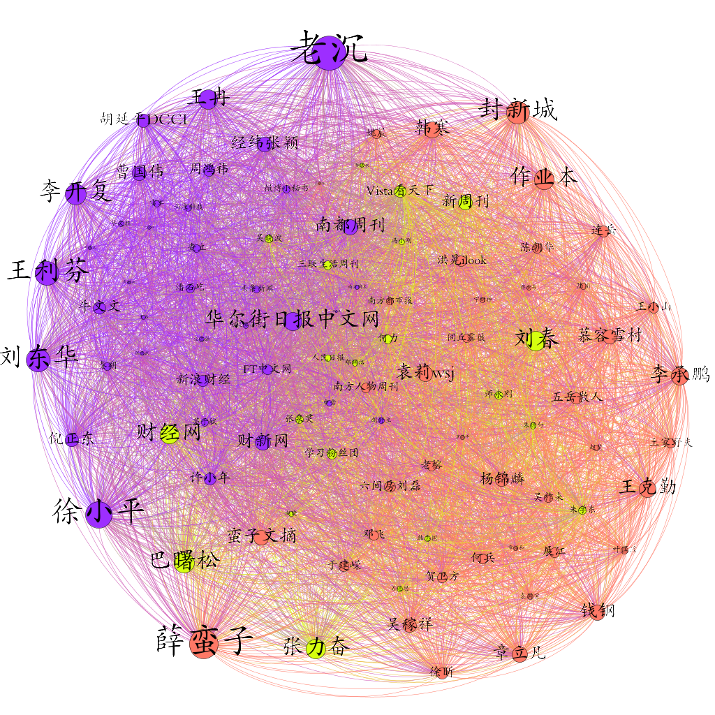
上一篇文章“Mahout与聚类分析”介绍了如何使用Mahout进行聚类分析的步骤，并且结合实例使用K-Means对微博名人共同关注数据进行了共被关注聚类分析。Mahout运行有本地运行和Hadoop运行两种模式，本地运行是指在用户本地的单机模式下运行，就像运行其他普通的程序一样，但是这样这样就不能最大限度的发挥出Mahout的优势，在本文中我们介绍如何让我们的Mahout聚类分析程序在Hahoop集群上运行（在实际操作中笔者使用的伪分布Hadoop，而不是真正的Hadoop集群）。

配置Mahout运行环境

Mahout运行配置可以在$MAHOUT_HOME/bin/mahout里面进行设置，实际上$MAHOUT_HOME/bin/mahout就是Mahout在命令行的启动脚本，这一点与Hadoop相似，但也又不同，Hadoop在$HADOOP_HOME\conf下面还提供了专门的hadoop-env.sh文件进行相关环境变量的配置，而Mahout在conf目录下没有提供这样的文件。

MAHOUT_LOCAL与HADOOP_CONF_DIR

以上的连个参数是控制Mahout是在本地运行还是在Hadoop上运行的关键。

$MAHOUT_HOME/bin/mahout文件指出，只要设置MAHOUT_LOCAL的值为一个非空（not empty string）值，则不管用户有没有设置HADOOP_CONF_DIR和HADOOP_HOME这两个参数，Mahout都以本地模式运行；换句话说，如果要想Mahout运行在Hadoop上，则MAHOUT_LOCAL必须为空。

HADOOP_CONF_DIR参数指定Mahout运行Hadoop模式时使用的Hadoop配置信息，这个文件目录一般指向的是$HADOOP_HOME目录下的conf目录。

除此之外，我们还应该设置JAVA_HOME或者MAHOUT_JAVA_HOME变量，以及必须将Hadoop的执行文件加入到PATH中。

综上所述：

1. 添加JAVA_HOME变量，可以在直接设置在$MAHOUT_HOME/bin/mahout中，也可以在user/bash profile里面设置(如./bashrc)

2. 设置MAHOUT_HOME并添加Hadoop的执行文件到PATH中

两个步骤在~/.bashrc的设置如下：

export JAVA_HOME=/usr/lib/jvm/java-7-openjdk-i386
#export HADOOP_HOME=/home/yoyzhou/workspace/hadoop-1.1.2
export MAHOUT_HOME=/home/yoyzhou/workspace/mahout-0.7
export PATH=$PATH:/home/yoyzhou/workspace/hadoop-1.1.2/bin:$MAHOUT_HOME/bin

编辑完~/.bashrc,重启Terminal即可生效。

3. 编辑$MAHOUT_HOME/bin/mahout，将HADOOP_CONF_DIR设置为$HADOOP_HOME\conf

HADOOP_CONF_DIR=/home/yoyzhou/workspace/hadoop-1.1.2/conf

读者可以将相关的Hadoop和Mahout主目录修改自己系统上面的目录地址，设置好之后重启Terminal，在命令行输入mahout，如果你看到如下的信息，就说明Mahout的Hadoop运行模式已经配置好了。

MAHOUT_LOCAL is not set; adding HADOOP_CONF_DIR to classpath. 
Running on hadoop...

要想使用本地模式运行，只需在$MAHOUT_HOME/bin/mahout添加一条设置MAHOUT_LOCAL为非空的语句即可。

Mahout命令行

Mahout为相关的数据挖掘算法提供了相应的命令行入口，同时提供了一些数据分析处理的用到的工具集。这些命令可以通过在终端输入mahout获得。以下显示了输入mahout的部分信息：

....
Valid program names are:
  arff.vector: : Generate Vectors from an ARFF file or directory
  baumwelch: : Baum-Welch algorithm for unsupervised HMM training
  canopy: : Canopy clustering
  cat: : Print a file or resource as the logistic regression models would see it
  cleansvd: : Cleanup and verification of SVD output
  clusterdump: : Dump cluster output to text
  ....
  fkmeans: : Fuzzy K-means clustering
  fpg: : Frequent Pattern Growth
  hmmpredict: : Generate random sequence of observations by given HMM
  itemsimilarity: : Compute the item-item-similarities for item-based collaborative filtering
  kmeans: : K-means clustering
....

Mahout kmeans

在上一篇文章，我们通过调用KMeansDriver.run()方法从Mahout程序中直接启动KMeans算法，这种方式对于在本地调试程序非常有用，但是在真实项目中，无论是使用Hadoop模式运行，还是本地运行，从命令行运行Mahout的相关算法更加合适，这样的好处是我们只需要给Mahout提供符合相应算法要求的输入数据，即可以利用Mahout分布式处理的优势。比如在本例中，使用kmeans算法，只需要事先将数据处理成Mahout kmeans算法要求的输入数据，然后在命令行调用mahout kmeans [options]即可。

在命令行输入不带任何参数的mahout kmeans，Mahout将为你列出在命令行使用kmeans算法的使用方法。

Usage:                                                                          
 [--input <input> --output <output> --distanceMeasure <distanceMeasure>         
--clusters <clusters> --numClusters <k> --convergenceDelta <convergenceDelta>   
--maxIter <maxIter> --overwrite --clustering --method <method>                  
--outlierThreshold <outlierThreshold> --help --tempDir <tempDir> --startPhase   
<startPhase> --endPhase <endPhase>]                                             
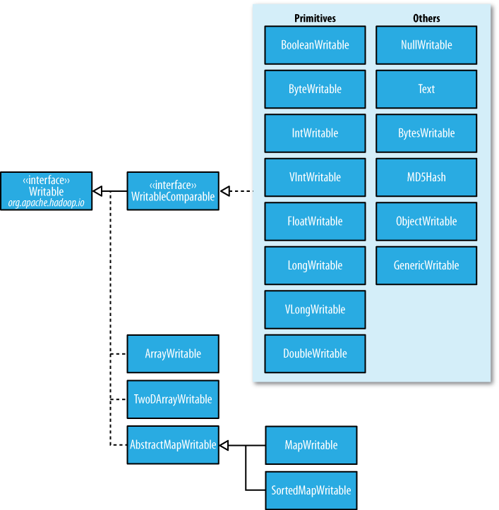
--clusters (-c) clusters    The input centroids, as Vectors.  Must be a         
	                        SequenceFile of Writable, Cluster/Canopy.  If k is  
	                        also specified, then a random set of vectors will   
	                        be selected and written out to this path first 

相关的参数我们已经在上篇文章中提到过。

具体的步骤如下：

1. 将数据处理为Mahout向量（Vector）的形式
2. 将Mahout向量转化为Hadoop SequenceFile
3. 创建K个初始质心\[可选\]
4. 将Mahout向量的SequenceFile复制到HDFS上
5. 运行`mahout kmeans [options]`

下面的命令显示使用CosineDistanceMeasure对data/vectors目录下Mahout向量数据进行kmeans聚类分析，输出结果保存在output目录下。

mahout kmeans -i data/vectors -o output -c data/clusters \
-dm org.apache.mahout.common.distance.CosineDistanceMeasure \
-x 10 -ow -cd 0.001 -cl

更加详细的命令行参数可以在Mahout wiki k-means-commandline上查找到。

总结

本文首先介绍了如何配置Mahout的Hadoop的运行环境，然后介绍如何使用mahout kmeans命令行将聚类分析运行在Hadoop上。

本文简要的介绍了Mahout以及聚类分析，并结合实例说明了如何使用Mahout的K-Means算法进行聚类分析。

Mahout

Mahout是Apache下的开源机器学习软件包，目前实现的机器学习算法主要包含有协同过滤/推荐引擎，聚类和分类三个部分。Mahout从设计开始就旨在建立可扩展的机器学习软件包，用于处理大数据机器学习的问题，当你正在研究的数据量大到不能在一台机器上运行时，就可以选择使用Mahout，让你的数据在Hadoop集群的进行分析。Mahout某些部分的实现直接创建在Hadoop之上，这就使得其具有进行大数据处理的能力，也是Mahout最大的优势所在。相比较于Weka，RapidMiner等图形化的机器学习软件，Mahout只提供机器学习的程序包（library），不提供用户图形界面，并且Mahout并不包含所有的机器学习算法实现，这一点可以算得上是她的一个劣势，但前面提到过Mahout并不是“又一个机器学习软件”，而是要成为一个“可扩展的用于处理大数据的机器学习软件”，但是我相信会有越来越多的机器学习算法会在Mahout上面实现。

聚类分析

物以类聚，人以群分。顾名思义，聚类分析就是将不同的对象分为不同的组或簇，它与我们日常生活所理解的类的概念是相一致的。聚类分析能够帮助我们很好地了解对象之间的类与结构，聚类分析也能够帮助我们将个别对象指派到相应的类。

聚类分析仅根据在数据中发现的描述对象及其关系的信息，将数据对象分组。其目标是，组内的对象相互之间是相似的（相关的），而不同组之间的对象是不同的（不相关的）。组内的相似性（同质性）越大，组间差别越大，聚类就越好。
《数据挖掘导论》 Pang-Ning Tan等

常见的聚类分析有K-Means聚类和层次聚类两种。此外还有基于密度的、基于图的以及基于模型的聚类分析方法。

从上面的定义中可以看出，聚类的分析的关键之一在于相似性的度量，常用的相似性有基于距离的相似度，余玄相似度，Jaccard相似度以及Pearson相关系数等。

Mahout聚类分析

Mahout的聚类分析提供了K-Means聚类、Fuzzy K-Means聚类和基于模型的聚类等方法。下面我们以K-Means聚类来说明如何使用Mahout进行聚类分析。

1. 数据准备

在进行数据分析时，第一步必然是准备分析数据。根据研究或者项目的要求收集数据，并且对数据进行必要的预处理。比如我下面我们要提到的微博用户共被关注分析中，首先我们要收集微博用户的关注信息，然后从关注信息中提取出用户共被关注的数据，也就是进行数据预处理。最终我们需要的数据可能就像下面的格式这样直白明确：“用户1,用户2,共被关注次数”。如果你是要进行文档的聚类分析，那么首先需要的获得的是文档的TF-IDF向量（文档-词向量）。

2. 将数据转换成Mahout中的Vector

Mahout要求每一个输入数据都应该是一个Vector，并且以Hadoop的SequenceFile类型存储。简单来说N维Vector就是一条N维记录，其中维就是记录的属性。比如一个TF-IDF向量就是一个文档记录，里面的属性就是词，有n个词就有n个维。有时候属性也叫特征。

在准备好Vectors之后，需要将这些记录写入到Hadoop Sequence文件中。下面的代码片段演示和如何创建Mahout Vector和将记录写成Sequence文件。

1
2
3
4
5
6
7
8
9
10
11
12
13
14
15
16
17
18
19
20
21
22
23
24
25
26
27
28
29
30
31
32
33
34

//...create Vector
//NamedVector is a Vector Wrapper class which owns a name for each vector, very convenient class 
NamedVector vec = new NamedVector(new RandomAccessSparseVector(cflist.size() + 1), account);
Iterator<CoFollowedNode> nodeItr = cflist.iterator();
while(nodeItr.hasNext()){
	CoFollowedNode cfnode= nodeItr.next();
	//set vector's n-dimension with co-followed number
	vec.set(cfnode.getDemension(), cfnode.getCoFollowedNum());
}


/**
  * Write Vectors to Hadoop sequence file, it's required per Mahout implementation that Vectors passed
  * into Mahout clusterings must be in Hadoop sequence file. 
  * 
  **/
private static void writeVectorsToSeqFile(ArrayList<NamedVector> vectors, String filename,
		FileSystem fs, Configuration conf) throws IOException {
		
	Path path = new Path(filename);
	SequenceFile.Writer writer = new SequenceFile.Writer(fs, conf, path,
				Text.class, VectorWritable.class);

		
	VectorWritable vec = new VectorWritable();
		
	//write vectors to file, the key is the account id, value is the co-followed vector of the key
	for (NamedVector entry : vectors) {
		vec.set(entry);
		writer.append(new Text(entry.getName()), vec);
	}
	writer.close();
		
}

3. 使用Mahout中的K-Means进行聚类

在介绍如何使用Mahout的K-Means之前，先复习一下基本的K-Means算法，如下所述：

**基本的K-Means算法**

1, 选择K个点作为初始质心

2, repeat:

3,	将每个点指派到最近的质心，形成K个簇

4,	重新计算每个簇的质心

5, until 质心不再发生改变

1
2
3
4
5
6
7
8
9
10
11
12
13
14
15
16
17

//write initial clusters point, in this case 5 points/vectors
Path path = new Path("data/clusters/part-00000");
SequenceFile.Writer writer = new SequenceFile.Writer(fs, conf, path,
		Text.class, Kluster.class);

for (int i = 0; i < k; i++) {
	NamedVector nVec =  vectors.get(i);
			
	Kluster cluster = new Kluster(nVec, i, new CosineDistanceMeasure());
	writer.append(new Text(cluster.getIdentifier()), cluster);
}
writer.close();
		
//here runs the k-means clustering in mapreduce mode, set runSequential to false
KMeansDriver.run(conf, new Path("data/vectors"), new Path(
		"data/clusters"), new Path("output"),
		new CosineDistanceMeasure(), 0.001, 10, true, 0, false);

上面的代码显示了Mahout中运行K-Means算法的用法，首先提供K个初始质心，如果用户没有提供初始质心，Mahout将根据用户给出的K随机的选择K个点作为初始质心。

KMeansDriver提供了运行K-Means算法的入口，其中的参数包含：

/**
   	* Iterate over the input vectors to produce clusters and, if requested, use the results of the final iteration to
   	* cluster the input vectors.
   	* 
   	* @param input
   	*          the directory pathname for input points
   	* @param clustersIn
   	*          the directory pathname for initial & computed clusters
   	* @param output
   	*          the directory pathname for output points
   	* @param measure
   	*          the DistanceMeasure to use
   	* @param convergenceDelta
   	*          the convergence delta value
   	* @param maxIterations
   	*          the maximum number of iterations
   	* @param runClustering
   	*          true if points are to be clustered after iterations are completed
   	* @param clusterClassificationThreshold
   	*          Is a clustering strictness / outlier removal parameter. Its value should be between 0 and 1. Vectors
   	*          having pdf below this value will not be clustered.
   	* @param runSequential
   	*          if true execute sequential algorithm, else run algorithm in mapreduce mode 
   	*/

总结

本文简要的介绍了Mahout以及聚类分析，并使用实例说明了如何使用Mahout的K-Means进行聚类分析。总的来说，使用Mahout进行聚类分析需要用户将数据转换成Mahout的Vector对象，并且写成Sequence文件格式，然后选择初始的质心和适当的距离度量调用KMeansDriver进行聚类。

当然聚类分析还有很多的内容，比如如何选择距离度量，K值如何确定以及如何度量聚类的好坏等等，本篇文章旨在介绍如何使用Mahout进行聚类分析，更多的关于聚类以及机器学习的知识请您阅读相关的专业书籍。

参考数目

[1] Sean Owen etc., Mahout in Action, Manning Publications, 2011

[2] Pang-Ning Tan等, 数据挖掘导论, 人民邮电出版社, 2011

[3] 文中代码实例的源码地址CoFollowedClustering.java

---EOF---

在前面两篇文章[1][2]中我们介绍了Hadoop序列化的相关知识，包括Writable接口与Writable对象以及如何编写定制的Writable类，深入的分析了Writable类序列化之后占用的字节空间以及字节序列的构成。我们指出Hadoop序列化是Hadoop的核心部分之一，了解和分析Writable类的相关知识有助于我们理解Hadoop序列化的工作方式以及选择合适的Writable类作为MapReduce的键和值，以达到高效利用磁盘空间以及快速读写对象。因为在数据密集型计算中，在网络数据的传输是影响计算效率的一个重要因素，选择合适的Writable对象不但减小了磁盘空间，而且更重要的是其减小了需要在网络中传输的数据量，从而加快了程序的速度。

在本文中我们介绍另外一种方法加快程序的速度，这就是使用RawComparator加速Hadoop程序。我们知道作为键（Key）的Writable类必须实现WritableComparable接口，以实现对键进行排序的功能。Writable类进行比较时，Hadoop的默认方式是先将序列化后的对象字节流反序列化为对象，然后再进行比较（compareTo方法），比较过程需要一个反序列化的步骤。RawComparator的做法是不进行反序列化，而是在字节流层面进行比较，这样就省下了反序列化过程，从而加速程序的运行。Hadoop自身提供的IntWritable、LongWritabe等类已经实现了这种优化，使这些Writable类作为键进行比较时，直接使用序列化的字节数组进行比较大小，而不用进行反序列化。

RawComparator的实现

在Hadoop中编写Writable的RawComparator一般不直接继承RawComparator类，而是继承RawComparator的子类WritableComparator，因为WritableComparator类为我们提供了一些有用的工具方法，比如从字节数组中读取int、long和vlong等值。下面是上两篇文章中我们定制的MyWritable类的RawComparator实现，定制的MyWritable由两个VLongWritable对组成，为了添加RawComparator功能，Writable类必须实现WritableComparable接口，这里不再展示实现了WritableComparable接口的MyWritableComparable类的全部内容，而只是MyWritableComparable类中Comparator的实现，完整的代码可以在github中找到。

1
2
3
4
5
6
7
8
9
10
11
12
13
14
15
16
17
18
19
20
21
22
23
24
25
26
27
28
29
30
31
32
33
34
35
36
37
38
39
40
41
42
43
44
45
46
47
48

...//omitted for conciseness
/**
 * A RawComparator that compares serialized VlongWritable Pair
 * compare method decode long value from serialized byte array one by one
 *
 * @author yoyzhou
 *
 * */
public static class Comparator extends WritableComparator {

	public Comparator() {
		super(MyWritableComparable.class);
	}

	public int compare(byte[] b1, int s1, int l1, byte[] b2, int s2, int l2) {

		int cmp = 1;
		//determine how many bytes the first VLong takes
		int n1 = WritableUtils.decodeVIntSize(b1[s1]);
		int n2 = WritableUtils.decodeVIntSize(b2[s2]);

		try {
			//read value from VLongWritable byte array
			long l11 = readVLong(b1, s1);
			long l21 = readVLong(b2, s2);

			cmp = l11 > l21 ? 1 : (l11 == l21 ? 0 : -1);
			if (cmp != 0) {

				return cmp;

			} else {

				long l12 = readVLong(b1, s1 + n1);
				long l22 = readVLong(b2, s2 + n2);
				return cmp = l12 > l22 ? 1 : (l12 == l22 ? 0 : -1);
			}
		} catch (IOException e) {
				throw new RuntimeException(e);
		}
	}
}

static { // register this comparator
	WritableComparator.define(MyWritableComparable.class, new Comparator());
}

...

通过上面的代码我们可以看到要实现Writable的RawComparator我们只需要重载WritableComparator的public int compare(byte[] b1, int s1, int l1, byte[] b2, int s2, int l2)方法。在我们的例子中，通过从VLongWritable对序列化后字节数组中一个一个的读取VLongWritable的值，再进行比较。

当然编写完compare方法之后，不要忘了为Writable类注册编写的RawComparator类。

总结

为Writable类编写RawComparator必须对Writable本身序列化之后的字节数组有清晰的了解，知道如何从字节数组中读取Writable对象的值，而这正是我们前两篇关于Hadoop序列化和Writable接口的文章所要阐述的内容。

通过以上的三篇文章，我们了解了Hadoop Writable接口，如何编写自己的Writable类，Writable类的字节序列长度与其构成，以及如何为Writable类编写RawComparator来为Hadoop提速。

参考资料

Tom White, Hadoop: The Definitive Guide, 3rd Edition

Hadoop序列化与Writable接口(一)

Hadoop序列化与Writable接口(二)

--EOF--

上一篇文章Hadoop序列化与Writable接口（一）介绍了Hadoop序列化，Hadoop Writable接口以及如何定制自己的Writable类，在本文中我们继续Hadoop Writable类的介绍，这一次我们关注的是Writable实例序列化之后占用的字节长度，以及Writable实例序列化之后的字节序列的构成。

为什么要考虑Writable类的字节长度

大数据程序还需要考虑序列化对象占用磁盘空间的大小吗？也许你会认为大数据不是就是数据量很大吗，那磁盘空间一定是足够足够的大，一个序列化对象仅仅占用几个到几十个字节的空间，相对磁盘空间来说，当然是不需要考虑太多；如果你的磁盘空间不够大，还是不要玩大数据的好。

上面的观点没有什么问题，大数据应用自然需要足够的磁盘空间，但是能够尽量的考虑到不同Writable类占用磁盘空间的大小，高效的利用磁盘空间也未必就是没有必要的，选择适当的Writable类的另一个作用是通过减少Writable实例的字节数，可加快数据的读取和减少网络的数据传输。

Writable类占用的字节长度

下面的表格显示的是Hadoop对Java基本类型包装后相应的Writable类占用的字节长度：

不同的Writable类序列化后占用的字数长度是不一样的，需要综合考虑应用中数据特征选择合适的类型。对于整数类型有两种Writable类型可以选择，一种是定长（fixed-length）Writable类型,IntWritable和LongWritable；另一种是变长（variable-length）Writable类型，VIntWritable和VLongWritable。定长类型顾名思义使用固定长度的字节数表示，比如一个IntWritable类型使用4个长度的字节表示一个int；变长类型则根据数值的大小使用相应的字节长度表示，当数值在-112～127之间时使用1个字节表示，在-112～127范围之外的数值使用头一个字节表示该数值的正负符号以及字节长度（zero-compressed encoded integer）。

定长的Writable类型适合数值均匀分布的情形，而变长的Writable类型适合数值分布不均匀的情形，一般情况下变长的Writable类型更节省空间，因为大多数情况下数值是不均匀的，对于整数类型的Writable选择，我建议：

1. 除非对数据的均匀分布很有把握，否则使用变长Writable类型

2. 除非数据的取值区间确定在int范围之内，否则为了程序的可扩展性，请选择VLongWritable类型

整型Writable的字节序列

下面将以实例的方式演示Hadoop整型Writable对象占用的字节长度以及Writable对象序列化之后字节序列的结构，特别是变长整型Writable实例，请看下面的代码和程序输出：

1
2
3
4
5
6
7
8
9
10
11
12
13
14
15
16
17
18
19
20
21
22
23
24
25
26
27
28
29
30
31
32
33
34
35
36
37
38
39
40
41
42
43
44
45
46
47
48
49
50
51
52
53
54
55
56
57
58
59
60
61
62
63
64
65
66
67
68
69
70
71
72
73
74
75
76
77
78
79
80
81
82
83
84
85
86

package com.yoyzhou.example;

import java.io.*;
import org.apache.hadoop.io.*;
import org.apache.hadoop.util.StringUtils;

/**
 * Demos per how many bytes per each built-in Writable type takes and what does
 * their bytes sequences look like
 * 
 * @author yoyzhou
 * 
 */

public class WritableBytesLengthDemo {

	public static void main(String[] args) throws IOException {

		// one billion representations by different Writable object
		IntWritable int_b = new IntWritable(1000000000);
		LongWritable long_b = new LongWritable(1000000000);
		VIntWritable vint_b = new VIntWritable(1000000000);
		VLongWritable vlong_b = new VLongWritable(1000000000);

		// serialize writable object to byte array
		byte[] bs_int_b = serialize(int_b);
		byte[] bs_long_b = serialize(long_b);
		byte[] bs_vint_b = serialize(vint_b);
		byte[] bs_vlong_b = serialize(vlong_b);

		// print byte array in hex string and their length
		String hex = StringUtils.byteToHexString(bs_int_b);
		formatPrint("IntWritable", "1,000,000,000",hex, bs_int_b.length);

		hex = StringUtils.byteToHexString(bs_long_b);
		formatPrint("LongWritable", "1,000,000,000",hex, bs_long_b.length);

		hex = StringUtils.byteToHexString(bs_vint_b);
		formatPrint("VIntWritable", "1,000,000,000",hex, bs_vint_b.length);

		hex = StringUtils.byteToHexString(bs_vlong_b);
		formatPrint("VLongWritable", "1,000,000,000", hex, bs_vlong_b.length);
		
		
	}

	private static void formatPrint(String type, String param, String hex, int length) {

		String format = "%1$-50s %2$-16s with length: %3$2d%n";
		System.out.format(format, "Byte array per " + type
				+ "("+ param +") is:", hex, length);

	}

	/**
	 * Utility method to serialize Writable object, return byte array
	 * representing the Writable object
	 * 
	 * */
	public static byte[] serialize(Writable writable) throws IOException {

		ByteArrayOutputStream out = new ByteArrayOutputStream();
		DataOutputStream dataOut = new DataOutputStream(out);
		writable.write(dataOut);
		dataOut.close();

		return out.toByteArray();

	}

	/**
	 * Utility method to deserialize input byte array, return Writable object
	 * 
	 * */
	public static Writable deserialize(Writable writable, byte[] bytes)
			throws IOException {

		ByteArrayInputStream in = new ByteArrayInputStream(bytes);
		DataInputStream dataIn = new DataInputStream(in);
		writable.readFields(dataIn);

		dataIn.close();
		return writable;

	}
}

程序输出：

Byte array per IntWritable(1,000,000,000) is:  \     
3b9aca00         with length:  4

Byte array per LongWritable(1,000,000,000) is: \     
000000003b9aca00 with length:  8

Byte array per VIntWritable(1,000,000,000) is: \     
8c3b9aca00       with length:  5

Byte array per VLongWritable(1,000,000,000) is:\    
8c3b9aca00       with length:  5

从上面的输出我们可以看出：

+ 对1,000,000,000的表示不同的Writable占用了不同字节长度

+ 变长Writable类型并不总是比定长类型更加节省空间，当IntWritable占用4个字节、LongWritable占用8个字节时，相应的变长Writable需要一个额外的字节来存放正负信息和字节长度。所以回到前面的整数类型选择的问题上，选择出最合适的整数Writable类型，我们应该对数值的总体分布有一定的认识。

Text的字节序列

可以简单的认为Text类是java.lang.String的Writable类型，但是要注意的是Text类对于Unicode字符采用的是UTF-8编码，而不是使用Java Character类的UTF-16编码。

Java Character类采用遵循Unicode Standard version 4的UTF-16编码[1]，每个字符采用定长的16位(两个字节)进行编码，对于代码点高于Basic Multilingual Plane(BMP，代码点U+0000～U+FFFF)的增补字符，采用两个代理字符进行表示。

Text类采用的UTF-8编码，使用变长的1～4个字节对字符进行编码。对于ASCII字符只使用1个字节，而对于High ASCII和多字节字符使用2～4个字节表示，我想Hadoop在设计时选择使用UTF-8而不是String的UTF-16就是基于上面的原因，为了节省字节长度/空间的考虑。

由于Text采用的是UTF-8编码，所以Text类没有提供String那样多的操作，并且在操作Text对象时，比如Indexing和Iteration，一定要注意这个区别，不过我们建议在进行Text操作时，如果可能可以将Text对象先转换成String，再进行操作。

Text类的字节序列表示为一个VIntWritable + UTF-8字节流，VIntWritable为整个Text的字符长度，UTF-8字节数组为真正的Text字节流。具体请看下面的代码片段：

1
2
3
4
5
6
7
8
9
10
11

...//omitted per conciseness
Text myText = new Text("my text");
byte[] text_bs = serialize(myText);
hex = StringUtils.byteToHexString(text_bs);
formatPrint("Text", "\"my text\"", hex, text_bs.length);
		
Text myText2 = new Text("我的文本");
byte[] text2_bs = serialize(myText2);
hex = StringUtils.byteToHexString(text2_bs);
formatPrint("Text", "\"我的文本\"", hex, text2_bs.length);
...

程序输出：

Byte array per Text("my text") is: \
 	076d792074657874 with length:  8

Byte array per Text("我的文本") is: \
0ce68891e79a84e69687e69cac with length: 13

在上面的输出中，首个字节代表的该段Text/文本的长度，在UTF-8编码下“my text”占用的字节长度为7个字节（07），而中文“我的文本”的字节长度是12个字节（0c）。

定制Writable类的字节序列

本节中我们将使用上篇文章中的MyWritable类进行说明，回顾一下，MyWritable是一个由两个VLongWritable类构成的定制化Writable类型。

1
2
3
4
5
6
7

...//omitted per conciseness
MyWritable customized = new MyWritable(new VLongWritable(1000),
 						new VLongWritable(1000000000));
byte[] customized_bs = serialize(customized);
hex = StringUtils.byteToHexString(customized_bs);
formatPrint("MyWritable", "1000, 1000000000", hex, customized_bs.length);
...

程序输出：

Byte array per MyWritable(1000, 1000000000) is: \
8e03e88c3b9aca00 with length:  8

从输出我们可以很清楚的看到，定制的Writable类的字节序列实际上就是基本Writable类型的组合，输出“8e03e88c3b9aca00”的前三个字节是1000的VLongWritable的字节序列，“8c3b9aca00”是1000000000VLongWritable的字节序列，这一点可以从我们编写的MyWritable类的write方法中找到答案：

1
2
3
4
5
6
7

...//omitted per conciseness
@Override
public void write(DataOutput out) throws IOException {
	field1.write(out);
	field2.write(out);
}
...

总结

本文通过实例介绍了Hadoop Writable类序列化时占用的字节长度，并分析了Writable类序列化后的字节序列的结构。需要注意的是Text类为了节省空间的目的采用了UTF-8的编码，而不是Java Character的UTF-16编码，自定义的Writable的字节序列与该Writable类的write()方法有关。

最后指出，Writable是Hadoop序列化的核心，理解Hadoop Writable的字节长度和字节序列对于选择合适的Writable对象以及在字节层面操作Writable对象至关重要。

参考资料

Tom White, Hadoop: The Definitive Guide, 3rd Edition

Hadoop序列化与Writable接口(一)

---EOF---

序列化

序列化（serialization）是指将结构化的对象转化为字节流，以便在网络上传输或者写入到硬盘进行永久存储；相对的反序列化（deserialization）是指将字节流转回到结构化对象的过程。

在分布式系统中进程将对象序列化为字节流，通过网络传输到另一进程，另一进程接收到字节流，通过反序列化转回到结构化对象，以达到进程间通信。在Hadoop中，Mapper，Combiner，Reducer等阶段之间的通信都需要使用序列化与反序列化技术。举例来说，Mapper产生的中间结果（<key: value1, value2...>）需要写入到本地硬盘，这是序列化过程（将结构化对象转化为字节流，并写入硬盘），而Reducer阶段读取Mapper的中间结果的过程则是一个反序列化过程（读取硬盘上存储的字节流文件，并转回为结构化对象），需要注意的是，能够在网络上传输的只能是字节流，Mapper的中间结果在不同主机间洗牌时，对象将经历序列化和反序列化两个过程。

序列化是Hadoop核心的一部分，在Hadoop中，位于org.apache.hadoop.io包中的Writable接口是Hadoop序列化格式的实现。

Writable接口

Hadoop Writable接口是基于DataInput和DataOutput实现的序列化协议，紧凑（高效使用存储空间），快速（读写数据、序列化与反序列化的开销小）。Hadoop中的键（key）和值（value）必须是实现了Writable接口的对象（键还必须实现WritableComparable，以便进行排序）。

以下是Hadoop（使用的是Hadoop 1.1.2）中Writable接口的声明：

1
2
3
4
5
6
7
8
9
10
11
12
13
14
15
16
17
18
19
20
21
22
23
24
25
26

package org.apache.hadoop.io;

import java.io.DataOutput;
import java.io.DataInput;
import java.io.IOException;

public interface Writable {
  /** 
   * Serialize the fields of this object to <code>out</code>.
   * 
   * @param out <code>DataOuput</code> to serialize this object into.
   * @throws IOException
   */
  void write(DataOutput out) throws IOException;

  /** 
   * Deserialize the fields of this object from <code>in</code>.  
   * 
   * <p>For efficiency, implementations should attempt to re-use storage in the 
   * existing object where possible.</p>
   * 
   * @param in <code>DataInput</code> to deseriablize this object from.
   * @throws IOException
   */
  void readFields(DataInput in) throws IOException;
}

Writable类

Hadoop自身提供了多种具体的Writable类，包含了常见的Java基本类型（boolean、byte、short、int、float、long和double等）和集合类型（BytesWritable、ArrayWritable和MapWritable等）。这些类型都位于org.apache.hadoop.io包中。

(图片来源：safaribooksonline.com)

定制Writable类

虽然Hadoop内建了多种Writable类提供用户选择，Hadoop对Java基本类型的包装Writable类实现的RawComparable接口，使得这些对象不需要反序列化过程，便可以在字节流层面进行排序，从而大大缩短了比较的时间开销，但是当我们需要更加复杂的对象时，Hadoop的内建Writable类就不能满足我们的需求了(需要注意的是Hadoop提供的Writable集合类型并没有实现RawComparable接口，因此也不满足我们的需要)，这时我们就需要定制自己的Writable类，特别将其作为键（key）的时候更应该如此，以求达到更高效的存储和快速的比较。

下面的实例展示了如何定制一个Writable类，一个定制的Writable类首先必须实现Writable或者WritableComparable接口，然后为定制的Writable类编写write(DataOutput out)和readFields(DataInput in)方法，来控制定制的Writable类如何转化为字节流（write方法）和如何从字节流转回为Writable对象。

1
2
3
4
5
6
7
8
9
10
11
12
13
14
15
16
17
18
19
20
21
22
23
24
25
26
27
28
29
30
31
32
33
34
35
36
37
38
39
40
41
42
43
44
45
46
47
48
49
50
51
52
53
54
55
56
57
58
59
60
61
62
63
64
65
66
67
68
69
70
71
72
73
74
75
76
77
78
79

package com.yoyzhou.weibo;

import java.io.DataInput;
import java.io.DataOutput;
import java.io.IOException;
import org.apache.hadoop.io.VLongWritable;
import org.apache.hadoop.io.Writable;

/**
 *This MyWritable class demonstrates how to write a custom Writable class 
 *
 **/
public class MyWritable implements Writable{
		
		
	private VLongWritable field1;
	private VLongWritable field2;
		
	public MyWritable(){
		this.set(new VLongWritable(), new VLongWritable());
	}
		
		
	public MyWritable(VLongWritable fld1, VLongWritable fld2){
			
		this.set(fld1, fld2);
			
	}
		
	public void set(VLongWritable fld1, VLongWritable fld2){
		//make sure the smaller field is always put as field1
		if(fld1.get() <= fld2.get()){
			this.field1 = fld1;
			this.field2 = fld2;
		}else{
				
			this.field1 = fld2;
			this.field2 = fld1;
		}
		}
				
	//How to write and read MyWritable fields from DataOutput and DataInput stream
	@Override
	public void write(DataOutput out) throws IOException {
			
		field1.write(out);
		field2.write(out);
	}

	@Override
	public void readFields(DataInput in) throws IOException {
			
		field1.readFields(in);
		field2.readFields(in);
	}

	/** Returns true if <code>o</code> is a MyWritable with the same values. */
	@Override
	public boolean equals(Object o) {
		 if (!(o instanceof MyWritable))
		    return false;
		
		    MyWritable other = (MyWritable)o;
		    return field1.equals(other.field1) && field2.equals(other.field2);
		
	}
		
	@Override
	public int hashCode(){
			
		return field1.hashCode() * 163 + field2.hashCode();
	}
		
	@Override
	public String toString() {
		return field1.toString() + "\t" + field2.toString();
	}
		
}

未完待续，下一篇中将介绍Writable对象序列化为字节流时占用的字节长度以及其字节序列的构成。

参考资料

Tom White, Hadoop: The Definitive Guide, 3rd Edition

---To Be Continued---

社交网络分析起源于社会学家使用数学与图论的方法研究社会群组中人与人之间的交互关系，如中心性分析、凝聚子群分析、社会结构分析等，最著名的莫过于美国社会心理学家Stanley Milgram的”六度分离理论”。传统的社会网络分析重点研究的是社会网络分析的概念以及通过社会网络分析研究社会结构对人、组织的影响，但是由于天然的地域限制，网络的大小受到一定的限制。

随着互联网的出现，特别是社交网站的迅速崛起，国外的Facebook、Twitter、Linked，国内的人人、微博等，互联网赋予了社交网络分析前所未有的机遇和新的挑战。首先，互联网打破了地域的限制，无论来自任何地方都可以通过互联网发生联系，目前Facebook有超过10亿的用户，他们来自全球，相互成为好友；其次，获得研究数据变得非常容易，社交网站拥有大量的用户数据，这些数据对社会网络分析来说就是宝贵的财富，以前从未有过，这也是目前社会网络分析在互联网爆发的主要原因；再次，相比于单一的人与人之间的交互关系，社交网站有着丰富的多媒体信息，除了用户关系，还有文本、图片、视频等内容。

但是数据不是信息，面对社交网站上的海量数据，需要有新的方法处理大数据，并从海量数据中挖掘出有价值的信息；同时应用社交网站的用户信息还面临这隐私保护的问题。

本文从社会网络分析的角度分析新浪微博名人帐号的关注网络，通过中介中心性分析关注网络中的控制网络信息流动的中心人物，并且使用Modularity（模块、群组）算法将关注网络划分为不同群组，最后我们使用Gephi可视化微博名人的关注网络。

相关理论简介

中介中心性

中介中心性（Betweenness Centrality）是处于网络中的点的中心性/重要程度的一种度量方式，网络中点的中介中心性直观的定义为“该点处于其他点最短路径上的次数”，处于这样位置上的点对路径上的信息传输具有一定的控制（阻止、掩饰、歪曲）能力。因此在同一个网络中，哪一个点的中介中心性越高，该点在网络中对信息的控制能力就越强，相反，中介中心性低，对信息的控制也就低。

如果希望了解中介中心性的详细内容，可参考Wikipedia上的词条Betweenness Centrality，和我的的上两篇文章A Set of Measures of Centrality Based on Betweenness与A Kinda Betweenness Centrality Algorithm。

网络群组

网络群组（Modularity）是社会网络分析中用于分析网络结构的一种方法。根据一个群组内部比群组外部具有更高密度的联结的原则，它将网络分成不同的群组（通常也叫群（groups）、族群（clusters）或者社群（communities）），通常用来侦测网络的社群结构。

更多群组的信息请参考Wikipedia词条Modularity.

数据来源

数据收集

本文所使用的数据来源于新浪微博的用户关注信息，一共收集了30999个新浪微博用户的关注信息，去重后被关注的用户数量为3,940,891位。

以下是收集数据的概述：

数据收集时间：2013.3.18~2013.4.2

原始数据：包含两部分，一部分是用户信息，另一部分是用户的关注信息

用户信息：用户信息从用户的/info页面上收集

用户关注信息：用户关注信息从用户的/follow页面逐页收集

数据预处理

首先，我们定义微博名人为：在我们所收集的数据中，被关注的次数大于等于1000；然后利用上小节中收集的数据，使用Hadoop将数据处理为：”用户, 关注用户”的形式。对于如何在Hadoop中使用Filter处理数据可以参考我的文章Adding Filter in Hadoop Mapper Class；最后我们获得了一个包含218,071个节点，677,268条边的微薄名人（有向）关注网络。

需要注意的是在下面的分析中，由于计算资源的有限，我们在Hadoop获得的结果上，进一步将节点数缩小到100个，相应的边的数量为4820。这一步骤是由限制名人网络中节点入度为178实现的。

微博名人关注网络分析

中介中心性和群组分析

下表列出了中介中心性Top20的微博名人（数据保留小数点后两位）。可以看出在我们的数据集中老沉（新浪执行副总裁、总编辑陈彤）、薛蛮子（著名天使投资人）和徐小平（真格基金创始人、新东方联合创始人）名列前三，李开复中心性值排在第七，为108.16；有11个账户的中介中心性值超过100，他们在网络中处于最短路径上的次数大于100。

上表中“群组”列给出了中心性Top20微博名人的群组分类，将他们大致分为三个群组：

+ 互联网+青年导师，

+ 新闻媒体相关，和

+ 新知识分子。

更直观的分类请参看下小节的可视化分析。

可视化分析

我们使用Gephi对微博名人关注网络数据进行可视化分析。如下图所示：

图中节点大小代表中介中心性的大小，节点的颜色代表相应的群组，相同的节点颜色表示处于同一个群组，从图中可以清楚的看到群组的分布情况。

动态交互网络：

动态交互网络/Interactive Dynamic Network

结束语

本文运用社会网络分析方法，通过中介中心性和群组两个维度，对微博名人的关注网络进行了分析，通过分析我们得出了微博名人中介中心性，并且将微博名人的关注网络划分为了三个群组。

虽然本文作者设想将本文作为大数据来进行分析，但是由于计算资源的有限，只能将分析的节点数一再降低；本文中对名人界定以数据集中被关注数量进行度量，更加准确的度量应该以现实微博中用户的被关注数量。

如何在MapReduce框架下进行社交网络分析，将会是一个很价值的主题。

最后，由于本文使用的数据是SINA微博用户数据的很小一部分，文中的排名和可视化网络并非SINA微博真实情况的反映，结论仅供参考。

---EOF---

In this post I’d like to demonstrate a algorithm per computing the betweenness centrality which I have introduced in the previous post, for more details of what is Betweenness Centrality, and its measurements, please refer to my post A Set of Measures of Centrality Based on Betweenness.

Definitions and notations

Before getting down to the algorithm, first we briefly go through the definitions and notations.

Betweenness Centrality is “the degree to which a point falls on the shortest path between others”, it’s the core of the algorithm. Although computing shortest path between point pair is essential to our problem, shortest path algorithm will not be the focus of this post. Readers interested in shortest path algorithm please refer to the shortest path on Wikipedia page here, kindly note that even if you have no knowledge of shortest path algorithm, it will not affect you reading this post.

In the next section, we use graph-theoretic terminology neutral to interpretation of notations.

Given a directed graph $\begin{smallmatrix} G = \left( V, E \right) \end{smallmatrix}$, consists of a set of $V$ of vertices and a set of $E \subseteq V \times V$ of derected edges.

Denote $\sigma(s, t)$ to the number of shortest $(s, t)$-paths, some times called geodesics, and let $\sigma(s,t \vert v)$ be the number of shortest path which passing through certain vertex $v$ other than $s, t$, then the betweenness centrality $C_B(v)$ of vertex $v \in V$ is defined to be:

The Algorithm

As quoted from “On variants of shortest-path betweenness centrality and their computation”:

Efficient computation of betweenness is based on the fact that the cubic number of pair-wise dependencies $\delta(s,t \vert v) = \sigma(s, t \vert v)/ \sigma(s, t)$ can be aggregated without computing all of them explicitly.

Defining one-side dependencies:

$\begin{align} \delta(s \vert v) = \sum\limits_{t \in V} \delta(s, t \vert v)\end{align}$,

per $\forall s, v \in V$ we can exploit that

where $dist(s, t)$ denotes the minimum path length of point pair $(s, t)$.

The algorithm asserts that the dependency of a vertex $s$ on some $v$ can be compiled from dependencies on vertices one edge farther away.

Since $w$ is connected to $v$ and one edge farther away (which determined by $dist(s, w) = dist(s, v) + 1$) from $v$, so point $v$ is on the shortest paths of $(s, w)$ and the proportion of betweenness value that $v$ gains from edge $(v, w)$ equals to $\frac{\sigma(s,v)}{\sigma(s, w)} \times 1$; the other part of betweenness gain is from point $w$, that $\frac{\sigma(s,v)}{\sigma(s, w)} \times \delta(s \vert w)$, thus sum of the above two parts of betweenness gain is what exactly the equation demonstrates.

References

[1] Linton C. Freeman. A set of measures of centrality based on betweenness. Sociometry, 40(1):35–41, March 1977.

[2] Ulrik Brandes. On variants of shortest-path betweenness centrality and their generic computation. Social Networks, 30(2):136–145, May 2008.

---EOF---

This post is a studying notes of paper “A Set of Measures of Centrality Based on Betweenness”, the paper [pdf], wrote by Freeman in 1977, is an introductory and the most classic paper of betweenness centrality. Based on the betweenness centrality concept first introduced by Bavelas in 1948, the paper introduces a set of measures of centrality, including point centrality, scale free (relative) point centrality, and graph centrality.

Betweenness and Point Centrality

The classical centrality measures of Bavelas (1950) etc. can not be used by unconnected networks, since they define the centrality of a point as the sum of the minimum distance between that point and all others, thus all distance sums are infinite in unconnected networks.

In order to obtain a more satisfactory solution per centrality measurements, Freeman adopts the betweenness concept first introduced by Bavelas, betweenness of a point is “the degree to which a point falls on the shortest path between others”, and therefore has a potential per control of communication, persons in such central positions could influence the group by “ withholding information (or) coloring, or distorting it in transmission”.

Measurement of Point Centrality

Consider a unordered pair of points {$p_i, p_j$} $(i \neq j)$. Either $p_i \text{ and } p_j$ are unreachable from each other or there are one or more paths between them. In the later case, each path has a length equals to the number of edges contained in it. Among the paths connecting pi and pj, one or more have the shortest length: the geodesics.

If $p_i$ and $p_j$ are unreachable from each other, then $b_{ij}(p_k)$, denotes betweenness centrality of point $p_k$ with respect to $p_i$ and $p_j$, is zero;

If $p_i$ and $p_j$ are adjacent, means that there is only one edge connecting them, since $p_k$ does not reside on the shortest paths of $p_i$ and $p_j$, $b_{ij}(p_k)$ also equals to zero;

If $p_k$ is on one or more shortest paths of $p_i$ and $p_j$, in which situations, $p_k$ has a proportional control of communication between $p_i$ and $p_j$, and intuitively the proportion is the percentage/extent to which $p_k$ is on the shortest paths, given the total shortest paths of $p_i$ and $p_j$ is $g_{ij}$ and the number of $p_k$ falls in the shortest paths is $g_{ij}(p_k)$, then we get $b_{ij}(p_k) = g_{ij}(p_k)/g_{ij}$. As the equation shows below:

To determine the overall centrality of $p_k$ in the graph, we need merely to sum the partial betweenness value of all unordered pair of points {$p_i, p_j$} in the graph:

Scale-free Point Centrality

One problem with the above point centrality is it not point independent/scale-free, it is related to how many points in the graph, thus comparing point centrality defined above with different graphs which may contain different amount of point is meaningless. A concreted example is pointed out that 6 betweenness value in 5 points graph compared with 6 betweenness value in 25 points graph, although they have the same betweenness centrality value but the influence of them is different.

In the later section Freeman introduced a relative point centrality, which is scale free to how many points in the graph, where point centrality $C'_B(p_k)$ is divided by the maximum centrality of their graph.

where $n$ is the number of points in the graph, and $\begin{smallmatrix} \text{Max } C_B(p_k^*) \end{smallmatrix}$ is only determined by n, which is $\begin{smallmatrix} \frac{n \times (n-1)}{2} - (n-1) = \frac{n^2 - 3n + 2}{2} \end{smallmatrix}$, therefore we obtain:

To get more information of how $\begin{smallmatrix} \text{Max } C_B(p_k^*) \end{smallmatrix}$ is computed, please refer to the paper for details, you can imagine such a point that stands on the shortest path of all other pairs of {$p_i, p_j$}, where $p_i$ and $p_j$ have merely one shortest path, such a graph looks like a star graph, that one point in the central and all others surround it.

Graph Centrality

Freeman defines the graph centrality as the average difference between the most central point and all others, which sounds like a little bit of information entropy, I think.

where $\begin{smallmatrix} C'_B(p_k^*) \end{smallmatrix}$ is the relative point centrality value of the most central point $p_k^*$ in the graph.

From the equation, we can see if all the points have the same centrality value then the graph centrality is 0; and if the graph is a star or wheel graph, then graph centrality is 1.

---EOF---

There is my solutions to tackle the disk spaces shortage problem I described in the previous post. The core principle of the solution is to reduce the number of output records at Mapper stage; the method I used is Filter, adding a filter, which I will explain later, to decrease the output records of Mapper, which in turn significantly decrease the Mapper’s Spill records, and fundamentally decrease the disk space usages. After applying the filter, with 30,661 records. some 200MB data set as inputs, the total Spill Records is 25,471,725, and it only takes about 509MB disk spaces!

Followed Filter

And now I’m going to reveal what’s kinda Filter it looks like, and how did I accomplish that filter. The true face of the FILTER is called Followed Filter, it filters users from computing co-followed combinations if their followed number does not satisfy a certain number, called Followed Threshold.

Followed Filter is used to reduce the co-followed combinations at Mapper stage. Say we set the followed threshold to 100, meaning users who doesn’t own 100 fans(be followed by 100 other users) will be ignored during co-followed combinations computing stage(to get the actual number of the threshold we need analyze statistics of user’s followed number of our data set).

Reason

Choosing followed filter is reasonable because how many user follows is a metric of user’s popularity/famousness.

HOW

In order to accomplish it, we need:

First, counting user’s followed number among our data set, which needs a new MapReduce Job;

Second, choosing a followed threshold after analyze the statistics perspective of followed number data set got in first step;

Third, using DistrbutedCache of Hadoop to cache users who satisfy the filter to all Mappers;

Forth, adding followed filter to Mapper class, only users satisfy filter condition will be passed into co-followed combination computing phrase;

Fifth, adding co-followed filter/threshold in Reducer side if necessary.

Outcomes

Here is the Hadoop Job Summary, after applying the followed filter with followed threshold of 1000, that means only users who are followed by 1000 users will have the opportunity to co-followed combinations, compared with the Job Summary in my previous post, most all metrics have significant improvements:

P.S.

Frankly Speaking, chances are I am on the wrong way to Hadoop Programming, since I’m palying Pesudo Distribution Hadoop with my personal computer, which has 4 CUPs and 4G RAM, in real Hadoop Cluster disk spaces might never be a trouble, and all the tuning work I have done may turn into meaningless efforts. Before the Followed Filter, I also did some Hadoop tuning like customed Writable class, RawComparator, block size and io.sort.mb, etc.

---EOF---

以下8个步骤是我在使用Eclipse开发MapReduce程序时的路线，假定读者已经配置好了Hadoop环境并且了解Eclipse的相关操作。

步骤0～4为在Eclipse中编写和调试MapReduce程序；步骤5、6为在伪分布模式下运行MapReduce程序，并且通过导出项目到指定目录实现了Eclipse项目与Hadoop的关联。

0 创建Java项目

1 在项目的CLASS PATH中添加Hadoop相关的JAR引用（注意在添加JAR文件，而不是JAR文件夹，要不然在4中会因为找不到JAR或者Class而报错）

如果你还下载了Hadoop的源码，也可以给Hadoop相关的JAR添加源码，这样在Eclipse就可以使用F3参看Hadoop源码）

2 按照MapReduce类规范，编写自己的MapReduce类

3 配置MapReduce类的运行参数

4 在Eclipse中以单机模式运行/调试程序

5 将程序导出（Export）为JAR文件到$HADOOP_HOME/lib下

6 在伪分布模式下运行程序 bin/hadoop jar lib/ur-exported-jar.JAR full-class-name 参数列表

例如，你导出的JAR文件名为myhadoop.jar，类名称com.coolcompany.wordcount，命令就是：bin/hadoop jar lib/myhadoop.jar com.coolcompany.wordcount 参数列表

7 部署程序到真实的Hadoop集群

---EOF---